


|
|
|
|
|
As you may have discovered, it is legal to make more than one assignment to the same variable. A new assignment makes an existing variable refer to a new value (and stop referring to the old value).
bruce = 5
print bruce,
bruce = 7
print bruce
The output of this program is 5 7, because the first time bruce is printed, his value is 5, and the second time, his value is 7. The comma at the end of the first print statement suppresses the newline after the output, which is why both outputs appear on the same line.
Here is what multiple assignment looks like in a state diagram:

With multiple assignment it is especially important to distinguish between an assignment operation and a statement of equality. Because Python uses the equal sign (=) for assignment, it is tempting to interpret a statement like a = b as a statement of equality. It is not!
First, equality is commutative and assignment is not. For example, in mathematics, if a = 7 then 7 = a. But in Python, the statement a = 7 is legal and 7 = a is not.
Furthermore, in mathematics, a statement of equality is always true. If a = b now, then a will always equal b. In Python, an assignment statement can make two variables equal, but they don't have to stay that way:
a = 5
b = a # a and b are now equal
a = 3 # a and b are no longer equal
The third line changes the value of a but does not change the value of b, so they are no longer equal. (In some programming languages, a different symbol is used for assignment, such as <- or :=, to avoid confusion.)
Although multiple assignment is frequently helpful, you should use it with caution. If the values of variables change frequently, it can make the code difficult to read and debug.
Computers are often used to automate repetitive tasks. Repeating identical or similar tasks without making errors is something that computers do well and people do poorly.
We have seen two programs, nLines and countdown, that use recursion to perform repetition, which is also called iteration. Because iteration is so common, Python provides several language features to make it easier. The first feature we are going to look at is the while statement.
Here is what countdown looks like with a while statement:
def countdown(n):
while n > 0:
print n
n = n-1
print "Blastoff!"
Since we removed the recursive call, this function is not recursive.
You can almost read the while statement as if it were English. It means, "While n is greater than 0, continue displaying the value of n and then reducing the value of n by 1. When you get to 0, display the word Blastoff!"
More formally, here is the flow of execution for a while statement:
The body consists of all of the statements below the header with the same indentation.
This type of flow is called a loop because the third step loops back around to the top. Notice that if the condition is false the first time through the loop, the statements inside the loop are never executed.
The body of the loop should change the value of one or more variables so that eventually the condition becomes false and the loop terminates. Otherwise the loop will repeat forever, which is called an infinite loop. An endless source of amusement for computer scientists is the observation that the directions on shampoo, "Lather, rinse, repeat," are an infinite loop.
In the case of countdown, we can prove that the loop terminates because we know that the value of n is finite, and we can see that the value of n gets smaller each time through the loop, so eventually we have to get to 0. In other cases, it is not so easy to tell:
def sequence(n):
while n != 1:
print n,
if n%2 == 0: # n is even
n = n/2
else: # n is odd
n = n*3+1
The condition for this loop is n != 1, so the loop will continue until n is 1, which will make the condition false.
Each time through the loop, the program outputs the value of n and then checks whether it is even or odd. If it is even, the value of n is divided by 2. If it is odd, the value is replaced by n*3+1. For example, if the starting value (the argument passed to sequence) is 3, the resulting sequence is 3, 10, 5, 16, 8, 4, 2, 1.
Since n sometimes increases and sometimes decreases, there is no obvious proof that n will ever reach 1, or that the program terminates. For some particular values of n, we can prove termination. For example, if the starting value is a power of two, then the value of n will be even each time through the loop until it reaches 1. The previous example ends with such a sequence, starting with 16.
Particular values aside, the interesting question is whether we can prove that this program terminates for all values of n. So far, no one has been able to prove it or disprove it!
As an exercise, rewrite the function nLines from Section 4.9 using iteration instead of recursion.
One of the things loops are good for is generating tabular data. Before computers were readily available, people had to calculate logarithms, sines and cosines, and other mathematical functions by hand. To make that easier, mathematics books contained long tables listing the values of these functions. Creating the tables was slow and boring, and they tended to be full of errors.
When computers appeared on the scene, one of the initial reactions was, "This is great! We can use the computers to generate the tables, so there will be no errors." That turned out to be true (mostly) but shortsighted. Soon thereafter, computers and calculators were so pervasive that the tables became obsolete.
Well, almost. For some operations, computers use tables of values to get an approximate answer and then perform computations to improve the approximation. In some cases, there have been errors in the underlying tables, most famously in the table the Intel Pentium used to perform floating-point division.
Although a log table is not as useful as it once was, it still makes a good example of iteration. The following program outputs a sequence of values in the left column and their logarithms in the right column:
x = 1.0
while x < 10.0:
print x, '\t', math.log(x)
x = x + 1.0
The string '\t' represents a tab character.
As characters and strings are displayed on the screen, an invisible marker called the cursor keeps track of where the next character will go. After a print statement, the cursor normally goes to the beginning of the next line.
The tab character shifts the cursor to the right until it reaches one of the tab stops. Tabs are useful for making columns of text line up, as in the output of the previous program:
1.0 0.0
2.0 0.69314718056
3.0 1.09861228867
4.0 1.38629436112
5.0 1.60943791243
6.0 1.79175946923
7.0 1.94591014906
8.0 2.07944154168
9.0 2.19722457734
If these values seem odd, remember that the log function uses base e. Since powers of two are so important in computer science, we often want to find logarithms with respect to base 2. To do that, we can use the following formula:
log2 x =
|
Changing the output statement to:
print x, '\t', math.log(x)/math.log(2.0)
yields:
1.0 0.0
2.0 1.0
3.0 1.58496250072
4.0 2.0
5.0 2.32192809489
6.0 2.58496250072
7.0 2.80735492206
8.0 3.0
9.0 3.16992500144
We can see that 1, 2, 4, and 8 are powers of two because their logarithms base 2 are round numbers. If we wanted to find the logarithms of other powers of two, we could modify the program like this:
x = 1.0
while x < 100.0:
print x, '\t', math.log(x)/math.log(2.0)
x = x * 2.0
Now instead of adding something to x each time through the loop, which yields an arithmetic sequence, we multiply x by something, yielding a geometric sequence. The result is:
1.0 0.0
2.0 1.0
4.0 2.0
8.0 3.0
16.0 4.0
32.0 5.0
64.0 6.0
Because of the tab characters between the columns, the position of the second column does not depend on the number of digits in the first column.
Logarithm tables may not be useful any more, but for computer scientists, knowing the powers of two is!
As an exercise, modify this program so that it outputs the powers of two up to 65,536 (that's 216). Print it out and memorize it.
The backslash character in '\t' indicates the beginning of an escape sequence. Escape sequences are used to represent invisible characters like tabs and newlines. The sequence \n represents a newline.
An escape sequence can appear anywhere in a string; in the example, the tab escape sequence is the only thing in the string.
How do you think you represent a backslash in a string?
As an exercise, write a single string thatproduces
this
output.
A two-dimensional table is a table where you read the value at the intersection of a row and a column. A multiplication table is a good example. Let's say you want to print a multiplication table for the values from 1 to 6.
A good way to start is to write a loop that prints the multiples of 2, all on one line:
i = 1
while i <= 6:
print 2*i, ' ',
i = i + 1
print
The first line initializes a variable named i, which acts as a counter or loop variable. As the loop executes, the value of i increases from 1 to 6. When i is 7, the loop terminates. Each time through the loop, it displays the value of 2*i, followed by three spaces.
Again, the comma in the print statement suppresses the newline. After the loop completes, the second print statement starts a new line.
The output of the program is:
2 4 6 8 10 12
So far, so good. The next step is to encapsulate and generalize.
Encapsulation is the process of wrapping a piece of code in a function, allowing you to take advantage of all the things functions are good for. You have seen two examples of encapsulation: printParity in Section 4.5; and isDivisible in Section 5.4.
Generalization means taking something specific, such as printing the multiples of 2, and making it more general, such as printing the multiples of any integer.
This function encapsulates the previous loop and generalizes it to print multiples of n:
def printMultiples(n):
i = 1
while i <= 6:
print n*i, '\t',
i = i + 1
print
To encapsulate, all we had to do was add the first line, which declares the name of the function and the parameter list. To generalize, all we had to do was replace the value 2 with the parameter n.
If we call this function with the argument 2, we get the same output as before. With the argument 3, the output is:
3 6 9 12 15 18
With the argument 4, the output is:
4 8 12 16 20 24
By now you can probably guess how to print a multiplication table by
calling printMultiples repeatedly with different arguments. In
fact, we can use another loop:
i = 1
while i <= 6:
printMultiples(i)
i = i + 1
Notice how similar this loop is to the one inside printMultiples. All we did was replace the print statement with a function call.
The output of this program is a multiplication table:
1 2 3 4 5 6
2 4 6 8 10 12
3 6 9 12 15 18
4 8 12 16 20 24
5 10 15 20 25 30
6 12 18 24 30 36
To demonstrate encapsulation again, let's take the code from the end of Section 6.5 and wrap it up in a function:
def printMultTable():
i = 1
while i <= 6:
printMultiples(i)
i = i + 1
This process is a common development plan. We develop code by writing lines of code outside any function, or typing them in to the interpreter. When we get the code working, we extract it and wrap it up in a function.
This development plan is particularly useful if you don't know, when you start writing, how to divide the program into functions. This approach lets you design as you go along.
You might be wondering how we can use the same variable, i, in both printMultiples and printMultTable. Doesn't it cause problems when one of the functions changes the value of the variable?
The answer is no, because the i in printMultiples and the i in printMultTable are not the same variable.
Variables created inside a function definition are local; you can't access a local variable from outside its "home" function. That means you are free to have multiple variables with the same name as long as they are not in the same function.
The stack diagram for this program shows that the two variables named i are not the same variable. They can refer to different values, and changing one does not affect the other.
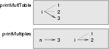
The value of i in printMultTable goes from 1 to 6. In the diagram it happens to be 3. The next time through the loop it will be 4. Each time through the loop, printMultTable calls printMultiples with the current value of i as an argument. That value gets assigned to the parameter n.
Inside printMultiples, the value of i goes from 1 to 6. In the diagram, it happens to be 2. Changing this variable has no effect on the value of i in printMultTable.
It is common and perfectly legal to have different local variables with the same name. In particular, names like i and j are used frequently as loop variables. If you avoid using them in one function just because you used them somewhere else, you will probably make the program harder to read.
As another example of generalization, imagine you wanted a program that would print a multiplication table of any size, not just the six-by-six table. You could add a parameter to printMultTable:
def printMultTable(high):
i = 1
while i <= high:
printMultiples(i)
i = i + 1
We replaced the value 6 with the parameter high. If we call printMultTable with the argument 7, it displays:
1 2 3 4 5 6
2 4 6 8 10 12
3 6 9 12 15 18
4 8 12 16 20 24
5 10 15 20 25 30
6 12 18 24 30 36
7 14 21 28 35 42
This is fine, except that we probably want the table to be
square with the same number of rows and columns. To do that, we
add another parameter to printMultiples to specify how many
columns the table should have.
Just to be annoying, we call this parameter high, demonstrating that different functions can have parameters with the same name (just like local variables). Here's the whole program:
def printMultiples(n, high):
i = 1
while i <= high:
print n*i, '\t',
i = i + 1
print
def printMultTable(high):
i = 1
while i <= high:
printMultiples(i, high)
i = i + 1
Notice that when we added a new parameter, we had to change the first line of the function (the function heading), and we also had to change the place where the function is called in printMultTable.
As expected, this program generates a square seven-by-seven table:
1 2 3 4 5 6 7
2 4 6 8 10 12 14
3 6 9 12 15 18 21
4 8 12 16 20 24 28
5 10 15 20 25 30 35
6 12 18 24 30 36 42
7 14 21 28 35 42 49
When you generalize a function appropriately, you often get a program with capabilities you didn't plan. For example, you might notice that, because ab = ba, all the entries in the table appear twice. You could save ink by printing only half the table. To do that, you only have to change one line of printMultTable. Change
printMultiples(i, high)
to
printMultiples(i, i)
and you get
1
2 4
3 6 9
4 8 12 16
5 10 15 20 25
6 12 18 24 30 36
7 14 21 28 35 42 49
As an exercise, trace the execution of this version of printMultTable and figure out how it works.
A few times now, we have mentioned "all the things functions are good for." By now, you might be wondering what exactly those things are. Here are some of them:
|
|
|
|
|